Bayesian Linear Regression Analysis (Insurance Premium Data)

---

Configuration

Import Library

library(rstan)
library(ggplot2)

• Apply STAN for analysis

Data Preprocessing

insdata=read.csv("insurance.csv")
insdata$sex <- ifelse(insdata$sex == "male", 0, 1)
insdata$smoker <- ifelse(insdata$smoker == "no", 0, 1)
# sex: male=0, female=1; smoker: no=0, yes=1

insdata=insdata[,c('age','sex','bmi','children','smoker','charges')]

• Translate the ‘sex’ variable into a binary format: male=0, female=1
• Translate the ‘smoker’ variable into a numeric format: False=0, True=1
• The ‘region’ variable is excluded from the analysis as it is categorical.
• Dependent variable: $log(charges)$, Independent variable: age, sex, bmi, children, smoker

Analysis

Linear regression with non-informative prior

model.reg1 = "
data {              
  int<lower=0> n;
  int<lower=0> p;
  matrix[n,p] X;
  vector[n] y;
}
parameters {            
  real alpha;
  vector[p] beta;
  real<lower=0> sigma_sq;  // error scale
}
model { 
  y ~ normal(X * beta + alpha, sqrt(sigma_sq));
  target += -log(sigma_sq);
}
"

sm=stan_model(model_code=model.reg1)
fit1 = sampling(
  object=sm,
  data=list(n=nrow(X), p=ncol(X), X=X, y=y),
  chains = 4,
  warmup = 2500,
  iter = 5000,
  cores = 4
)

beta.hat=get_posterior_mean(fit1,par="beta")[,"mean-all chains"]
alpha.hat=get_posterior_mean(fit1,par="alpha")[,"mean-all chains"]

aggregate(y-(alpha.hat+as.matrix(X)%*%beta.hat), list(group), FUN=var)

• Since there is no information about the population, a non-informative prior is employed for conducting linear regression analysis.
• MCMC sample count = $chains * (iter-warmup) / thin = 4 * (5000-2500)/1 = 10,000$

print(fit1)

• With a chain count of 4 and all parameters having an Rhat value of 1, the MCMC has converged.

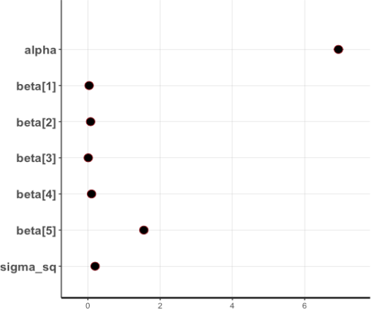
plot(fit1)

• It is possible to examine the posterior mean of each parameter.
  – age: 0.03, sex: 0.08, bmi: 0.01, children: 0.10, smoker: 1.55
• It is possible to examine the 95% CI of each parameter.
  – age: (0.03, 0.04), sex: (0.03, 0.12), bmi: (0.01, 0.01), children: (0.08, 0.12), smoker: (1.49, 1.61)

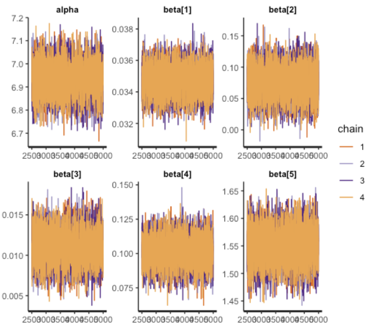
traceplot(fit1,pars=c("alpha","beta"))

• During the chain iteration process, parameters display no persistent long-term trends in their fluctuations. Mean values maintain stability as they converge towards a stationary distribution. This trait serves as an indicator of the MCMC chain’s favorable quality.

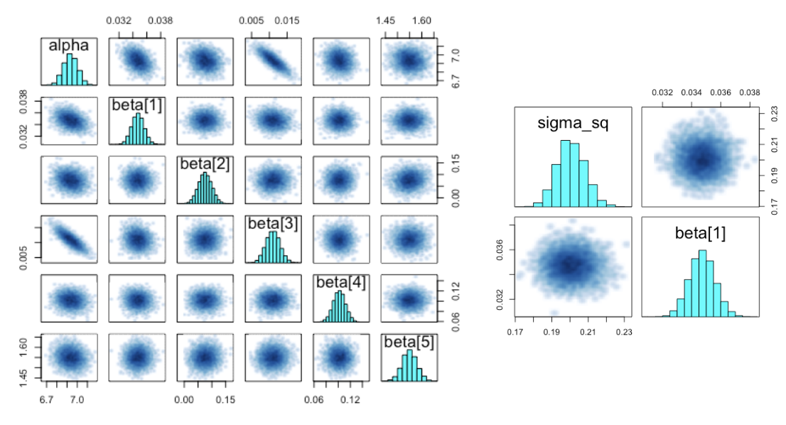
pairs(fit1,pars=c("sigma_sq","beta[1]"))

• Distribution of Posterior Distribution Density

Linear regression with informative prior

model.reg2="
data {
  int<lower=0> n;
  int<lower=1> p;
  int<lower=1> J;
  int<lower=1,upper=J> G[n];
  matrix[n, p] X;
  vector[n] y;
  vector[p] b0;
  matrix[p,p] Sig0;
}
parameters {
  real alpha;
  vector[p] beta;
  vector<lower=0>[J] sigma_sq; 
}
model {
  alpha ~ normal(0, 100);
  beta ~ multi_normal(b0,Sig0);
  for (j in 1:J) {
    sigma_sq[j] ~ inv_gamma(0.001, 0.001);
  }
  for (i in 1:n) {
    y[i] ~ normal(alpha+X[i]*beta, sqrt(sigma_sq[G[i]]));
  }
}
"

sm=stan_model(model_code=model.reg2)
fit2 = sampling(
  object=sm,
  data=list(n=nrow(X), p=ncol(X), J=length(table(group)), G=group, X=X, y=y, b0=rep(0,ncol(X)),Sig0=1000*diag(ncol(X))),
  chains = 4,
  warmup = 2500,
  iter = 5000,
  cores = 4
)

• The age groups were segmented into their respective 10s, 20s, 30s, 40s, and 50s categories, and a regression model was fitted using an informative prior.
• MCMC sample count = $chains * (iter-warmup) / thin = 4 * (5000-2500)/1 = 10,000$

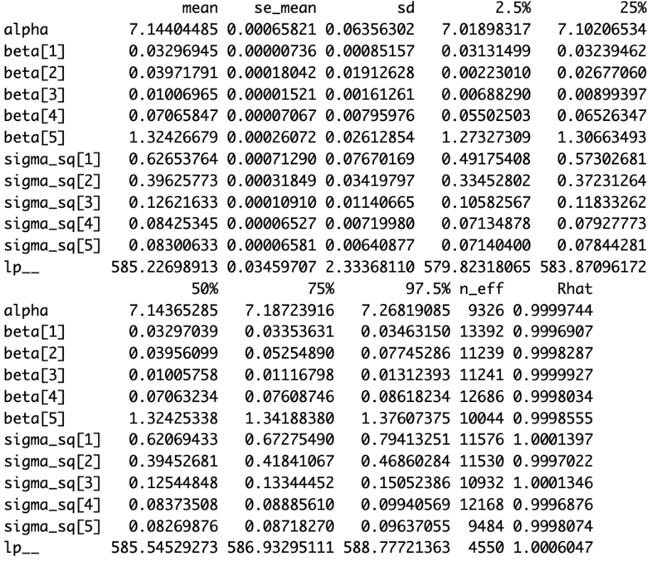
print(fit2,digits_summary=8)

• It is possible to examine the posterior mean of each parameter.
  – age: 0.03, sex: 0.04, bmi: 0.01, children: 0.07, smoker: 1.32
• It is possible to examine the 95% CI of each parameter.
  – age: (0.031, 0.035), sex: (0.002, 0.077), bmi: (0.007, 0.013), children: (0.055, 0.086), smoker: (1.273, 1.376)
• With a chain count of 4 and Rhat values close to 1, the MCMC has converged.

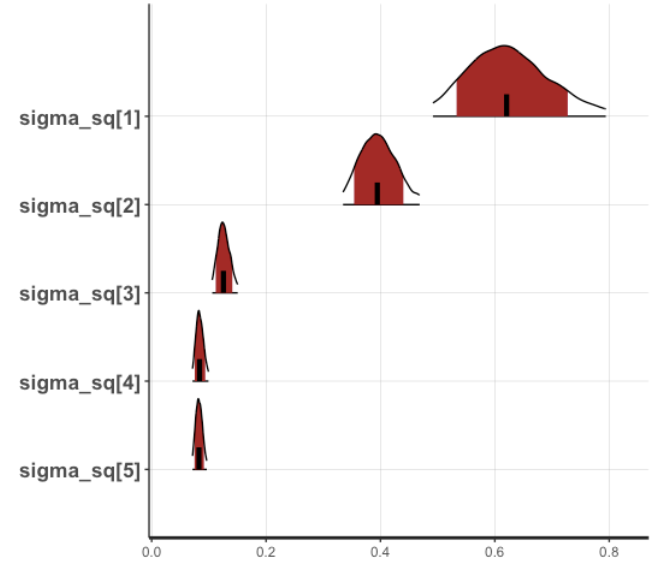
plot(fit2, pars="sigma_sq", show_density = TRUE)

• Distribution of Posterior Distribution Density

결과

The final regression equation $ log(charges) = 7.144 + 0.033 * 𝑎𝑔𝑒 + 0.040* 𝑠𝑒𝑥 + 0.010 * 𝑏𝑚𝑖 + 0.071 * 𝑐h𝑖𝑙𝑑𝑟𝑒𝑛 + 1.324 * 𝑠𝑚𝑜𝑘𝑒𝑟 $