[DACON] Credit Card Delinquency Level Prediction(LightGBM)

---

Introduction

Credit card companies use personal information and data submitted by credit card applicants to calculate credit scores.
They use this credit score to predict the applicant’s likelihood of defaulting on future payments and delinquent credit card payments.
In this project, we develop an algorithm that can predict the degree of delinquency of a user’s credit card payment using personal information data of credit card users.

Experiment

1. Data Preparation

1.1. Data Exploration

There are 20 columns including index and credit(dependent variable).

Feautre	Format	Description
index
gender	object	M: Male / F: Female
car	object	have car or not(Y/N)
reality	object	have reality or not(Y/N)
child_num	integer	number of children
income_total	float(0.0)	annual income
income_type	object	Commercial associate, Working, State servant, Pensioner, Student
edu_type	object	Higher education, Secondary / secondary special, Incomplete higher, Lower secondary, Academic degree
family_type	object	Married, Civil marriage, Separated, Single / not married, Widow
house_type	object	Municipal apartment, House / apartment, With parents, Co-op apartment, Rented apartment, Office apartment
DAYS_BIRTH	integer	interval between data collection date and birth date(negative number)
DAYS_EMPLOYED	integer	interval between data collection date and first working date(negative number)
FLAG_MOBIL	integer	have cell phone or not(1/0)
work_phone	integer	have business cell phone or not(1/0)
phone	integer	have phone or not(1/0)
email	integer	have email or not(1/0)
occyp_type	object	type of occupation(NaN)
family_size	float(0.0)	number of family member
begin_month	float(0.0)	interval between data collection date and card issue date(negative number)
credit	float(0.0)	credit card delinquency level(lower credit means better user

1.2. Data Preprocessing

I need to drop unusable variable(index) and fill NaN cells with None.
I then simplify the dependent variable by redefining the 3 levels of credit to 2 levels.(float → category)

df.drop(columns=['index'], inplace=True) # df: pandas dataframe of credit card data
df['occyp_type'] = df['occyp_type'].fillna('None')
df['credit'] = df['credit'].map(lambda x: 'low_risk' if x<=1.0 else 'high risk').astype('category')

Since categorical variables cannot be used in LightGBM, the category data type must be converted to object.

cat_vars = list(df.select_dtypes('object').columns)
df[cat_vars] = df[cat_vars].astype('category')

2. Model Fitting

2.1. Model Optimization

First, the data set is divided into independent and dependent variables, and then divided into train and test data in a ratio of 7:3 in a fixed random state 2021.

y = df['credit']
x = df.drop(columns=['credit'])
x_train, x_test, y_train, y_test = train_test_split(x, y, test_size=0.3, random_state=2021)

Next, the model parameters are optimized using the 5-fold algorithm with the train data./ The evaluation indicator at this project is logloss.

# Evaluation Indicator
logloss_ = make_scorer(log_loss, greater_is_better=False, needs_proba=True)

# LightGBM
warnings.filterwarnings("ignore")
md_lgb = LGBMClassifier(random_state=2021, categorical_feature=cat_vars)

# Parameter Optimization
params_lgb = {
    'learning_rate':[0.05, 0.1, 0.15],
    'n_estimators':[100, 200, 300, 400],
    'max_depth':[5, 6, 7, 8, 9],
    'num_leaves':[31, 47, 63],
    'reg_alpha':[0, 1],
    'reg_lambda':[0, 1, 10]
}

grid_search_lgb = RandomizedSearchCV(estimator=md_lgb, 
                                     param_distributions=params_lgb,
                                     n_iter=10,
                                     cv=5, 
                                     scoring=logloss_, 
                                     random_state=2021)

grid_search_lgb.fit(x_train, y_train, categorical_feature=cat_vars)

# Show Result
print(grid_search_lgb.best_params_)
print(grid_search_lgb.best_score_)

The result be like this.

• {‘reg_lambda’: 1, ‘reg_alpha’: 0, ‘num_leaves’: 47, ‘n_estimators’: 400, ‘max_depth’: 9, ‘learning_rate’: 0.05}
• -0.5505740190402201

Using these parameters, the model can be optimized.

# Model Optimization
md_lgb_best = LGBMClassifier(random_state=2021,
                             reg_lambda=1,
                             num_leaves=47,
                             max_depth=9,
                             learning_rate=0.05)

md_lgb_best.fit(x_train, y_train,
               categorical_feature=cat_vars,                
                eval_set=[(x_test, y_test)],
                early_stopping_rounds=10)

2.2. Model Evaluation

log_loss(y_test, md_lgb_best.predict_proba(x_test))

• 0.552121430722158

3. Conclusion

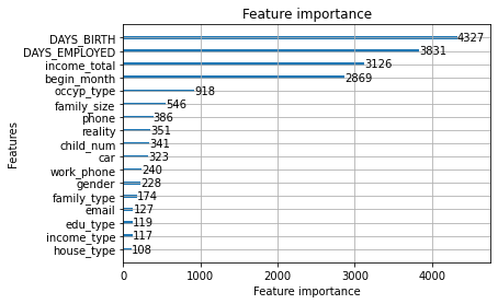
The importance of variables in the model is as follows.

plot_importance(md_lgb_best)
plt.show()

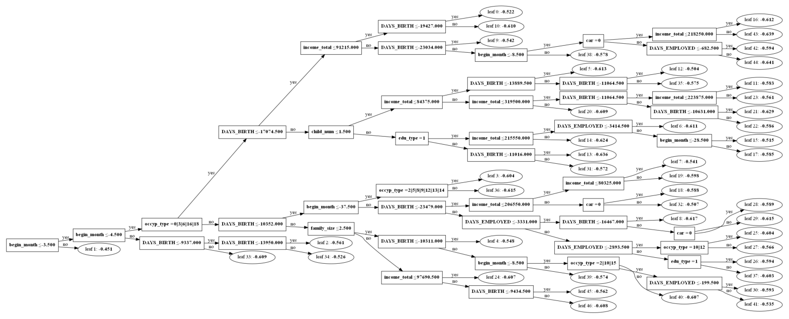
This is the visualized appearance of tree 0.

plot_tree(md_lgb_best, tree_index=0, dpi=100, figsize(20,12))
plt.show()

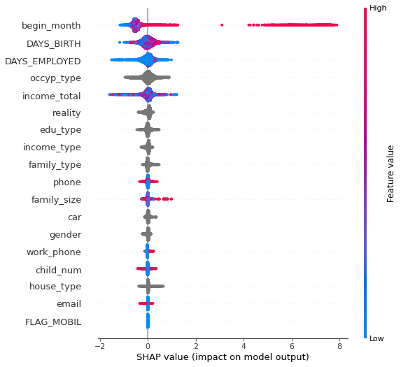
Next, calculate SHAP and look at the SHAP distribution for each variable.

explainer = shap.TreeExplainer(md_lgb_best)
shap_values = explainer.shap_values(x_test)
shap.initjs()
shap.summary_plot(shap_values[1], x_test, feature_names = x_test.columns)